How does a statistical test work? – Part 1

When you do your first statistical tests you may get the impression that doing statistics is complicated. There are so many variables and values, a level of significance, a p-value a t-value or F-value and much more. Here we want to show that the principle of statistical testing is actually relatively simple.
Statistical tests are generally based on two steps:

1. Calculation of a test statistic (using our data and a formula)
2. Comparison of the test statistic with a threshold value (using the distribution of the respective test statistic)

Step 1 – Calculation of a test statistic

Let’s have a look at step 1: A test statistic is a value calculated using our data according to a formula which somebody invented or which was derived based on mathematical considerations. Let’s have a look at the Student’s t-test as an example, which is used to compare two groups. A typical example for using t-test would be the comparison of body weight in adults to answer the question if there is a difference between the weight of women and men. The first step of the t-test is the calculation of the “test statistic”, which in the case of t-test is called “t-statistic”. In the case of the t-statistic, a formula is used, which has been based on the assumption that data are normally distributed:

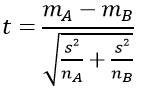
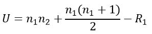
We use this formula to calculate a t-statistic (or a “t-value”) from our measured data. We don’t need to worry about the details of the formula now. To understand the principle of a statistical test, it’s enough to know that a test statistic is somehow calculated using a formula. If we look at another test, for example Mann-Whitney-U-test, then the name for the test statistic is different and another formula is used, but the main principle is the same: We calculate a test statistic. For the Mann-Whitney-U-test, the test statistic is not called t but called “U-statistic“ – as you may have expected, since we are talking about Mann-Whitney-U-test:

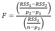
Let’s see another example: Fishers F-test. The test statistic for F-test is called F-statistic and this is the formula:

Step 2 – Comparison of the test statistic with a threshold value

So what do we do with this test statistic, calculated from our data and a given formula? The key idea of the next step is the following: Let’s consider we take two samples from the same pool of data (or as a statistician would say, from the same “population”). Then there should in principle be no difference between these two samples. Of course when we pick e.g. 20 random values from the same pool there will be some variation by chance (=some stochastic variability, as statisticians would say), but overall we should obtain two very similar samples, with a similar mean and standard deviation. From these two samples we can calculate our test statistic.

Evaluate your test statistic: The t-distribution

For example, for a t-test we can calculate the t-statistic. Now this t-statistic describes a situation where in principle there was no difference between the two samples. Now we can repeat the whole process and take another two samples and calculate a t-value. And then we do it again and again. After repeating this process many times, we have obtained many t-values, all describing a situation where there was no difference between the two samples. If we plot all these t-values into a graph, we can see how they are distributed:

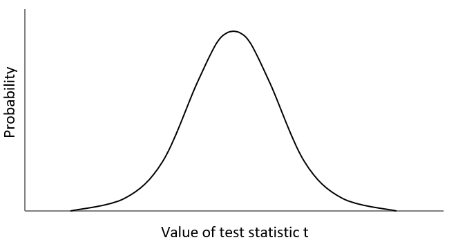
On the x-axis of this graph we see the value of the test statistic t. On the y-axis we see how often a value occurred, i.e. the probability of observing a given t-value. For example, a t-value from the centre of this distribution was observed more often (=it has a high probability). A value from the tails of the distribution (on the left and right) was observed only rarely (=it has a low probability). Hence, this so called “t-distribution” represents t-values which were all obtained when there was no difference between our two samples. Now how can we perform an actual statistical test?

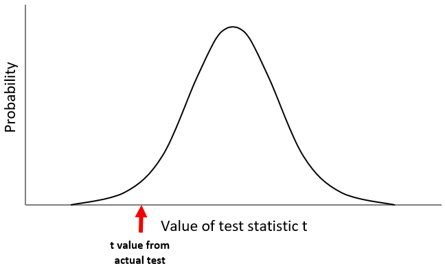
Evaluate your test statistic: The t-value

We take the actual samples for which we wanted to know whether there differ or not and then calculate a t-value. Imagine we had obtained a t-value near the left tail of the distribution (the red arrow in the graph below):

How can decide if the observed difference between the groups is random or not, i.e. if the difference between our two samples is statistically significant? Well, the question is “how certain do you want to be that the difference is not random?” Typically, we want to be quite certain, that means we only want to accept that a difference is not random, when we are very, very sure. More exactly: 95% sure.

Evaluate your test statistic: The level of significance

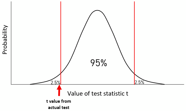
This is why we usually use a level of significance of α = 0.05 (when our p-value is below α we decide that a difference is significant). Hence we accept that a difference as being “statistically significant” when the risk for error is only 5% (which is expressed by the level of significance of α = 0.05). So we want to be 95% sure that a difference is not random. Now the t-distribution comes again into play: we can look at the x-axis and try to find the point where 95% of t values are higher and 5% are lower. This is illustrated in the graph by the red line:

The meaning of significance

This line represents a threshold with which we can compare the test statistic t, which we calculated from our two samples. Since this t-value is lower than the threshold, we can conclude that we have a significant difference between the two groups. We could also express this in different ways: For example:

We can be more than 95% sure that there is a difference between our samples.

Or:

The probability to observe a t value from two samples which are not different is lower than 5%.

Maybe this latter sentence also helps to understand the way how statisticians think: We actually started building a t-distribution which describes the case that there are no differences between our samples. This was our “hypothesis” (in statistical terms: our “Null hypothesis”). And now, when comparing the t value from the actual statistical test with two samples, for which we want to know if there is a difference or not, we reject this hypothesis.

In summary, statistical tests follow the two steps:

1. Calculation of a test statistic (using our data and a formula)
2. Comparison of the test-statistic with a threshold value (using the distribution of the respective test statistic)

One-sided vs. two-sided tests

While the description above correctly describes how statistical tests work, there are some points we didn’t mention so far to keep things simple: What we actually did was a “one-sided test”. A one-sided test is a test where we only test if one sample is on average lower than the other. For example, we want to know if one group is heavier than the other. Another word for a one-sided test is “one-tailed test” and this term refers to the distribution, where we only looked at one “tail”.

Now how about two-tailed tests (or two-sided tests)? The principle is the same but now we have two thresholds, one on the left and one on the right:

95% of t values are located between the two thresholds, so the level of significance α still is 5% or 0.05. But now we reject the hypothesis “no difference between the two groups” either when our test statistic is below the lower threshold or when it is above the upper threshold. In this case here, we can see that the arrow (our t value) is still below the lower threshold, hence we still conclude that there is a statistically significant difference between the groups.

Summary

So this is the relatively simple principle of statistical tests. We first calculate a test statistic and then we compare this value with the threshold of the distribution of the test statistic. This distribution describes all values of the test statistic when there is no difference between samples. For two-sided tests we use two thresholds.